Deep Generative Adversarial Networks for Thin-Section Infant MR Image Reconstruction
Jiaqi Gu1, Zezu Li1, YuanYuan Wans1, 3, Haowei Yang2, Zhongwei Qiao2, and Jinhua Yu1, 3
1School of Information Science and Technology, Fudan University, Shanghai 200433, China
Abstract
Thin section magnetic resonance images (Thin MRI ) 는 뇌수술, 뇌 구조 분석에 좋은 영상.
하지만 Thick section magnetic resonance images (Thick MRI ) 에 비해 imaging cost가 많이 들기 때문에 잘 사용되지 않음.
Thick MRI 2 Thin MRI 제안.
Two stage( GAN -> CNN )로 구성하였고 Thick MRI의 Axial, Sigittal plane을 이용하여 Thin MRI의 Axial reconstruction.
3D-Y-Net-GAN 은 Axial, Sagittal Thick MRI 를 이용하여 Fusion.
3D-Dense U-Net은 Sagittal plane에 대해 세부적인 calibrations, structual correction 제공.
Loss function 은 structual detail을 Network가 capture 할 수 있도록 제안.
bicubic, sparse representation, 3D-SRU-Net 과 비교.
35번의 Cross-validation, 114개를 이용하여 두개의 testset 구성.
PSNR : 23.5 % 증가.
SSIM : 90.5 % 증가.
MMI : 21.5 % 증가.
Introduction
Thin MRI 는 slice thickness가 1mm이고 sapcing gap이 0mm.
하지만 항상 Thin MRI를 사용할 수 없음.
일반적으로 사용하는 Thick MRI는 slice thickness가 4~6mm 이고 sapcing gap이 0.4~1mm.
해상도 : Thin MRI > Thick MRI
인간의 뇌 발달에 대한 insight를 주기 때문에 유아의 brain MR image는 어른의 brain MR image 보다 연구에 가치가 있음
하지만 유아의 MR image를 얻는게 쉽지 않음.
그래서 Thick to Thin 제안.
기존 traditional interpolation algorithm
Frame interpolation 방법과 같이 적용 가능.
Super-resolution 문제로 적용할 수도 있음.
CNN, GAN 이 발전하면서 super-resolution 이 탄력을 받음.
이전에 성인의 Thick MRI를 Thin MRI 로 reconstruction 하는 3D-SRGAN 제안했으나 axial plane만 고려했음. [Reconstruction of Thin-Slice Medical Images Using Generative Adversarial Network ]
Deep Learning 이 reconstruction performance 뿐 아니라 reconstruction time 감소에도 매우 효과적인걸 보임.
Proposed Method
A. Overview
CNN은 기존에도 super-resolution에서 많이 사용됨.
하지만 최근까지 제안된 Network는 대부분 2D image에 대한 upscaling.
몇몇 Network는 3D image로 확장했지만 그렇게 효과를 보지 못했음.
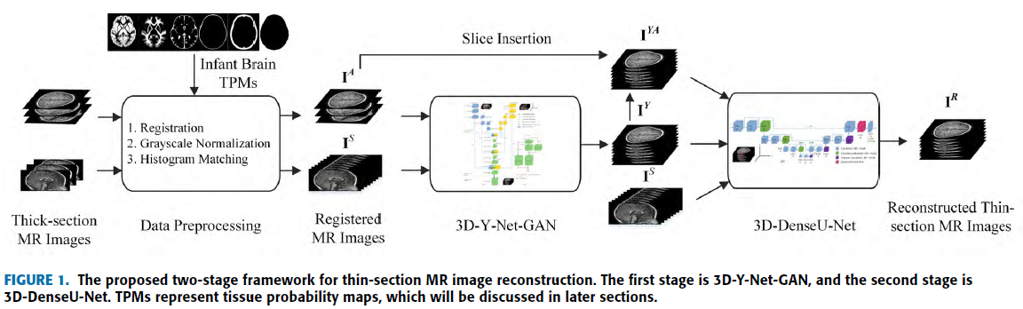
이 논문의 Flow
B. Network Architecture
First stage는 3D-Y-Net-GAN 으로 Thick MRI를 Thin MRI로 생성 후 3D-DenseU-Net으로 recalibration.
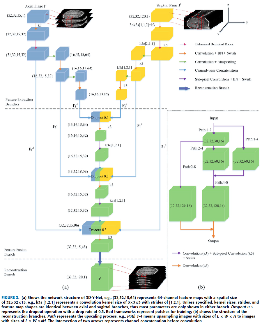
3D-Y-Net-GAN
Input : Axial, Sagittal Thick MRI
Output : Thin MRI
r : Upscaling Factor ( r = 8 일 경우의 예시 )
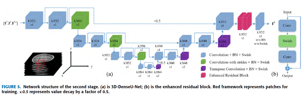
3D-DenseU-Net
전체적인 구조는 U-Net이지만 2개의 Enhanced residual block 을 적용하여 detail recalibration.
Input : \(I^Y, I^S, I^{YA}\) -> 어떻게 3개가 input으로…?
Output : Thin MR Image
\(I^A\) 를 \(I^Y\) 의 해당 위치에 insertion 하여 \(I^{YA}\) 생성. -> 아직 이해 X..
Axial Information 을 이용하여 정확한 axial 을 만들기 위해…
\(I^S\) 를 \(I^Y\) 에 insertion하게 되면 Sagittal 에 대한 information 이 과해지기 때문에 Reconstrtion Axial Image의 Quality 가 안좋아 질 것!
End-to-End 가 아니라 각각 따로따로 학습. -> Faster RCNN 과 같은 방식으로 할런지….?
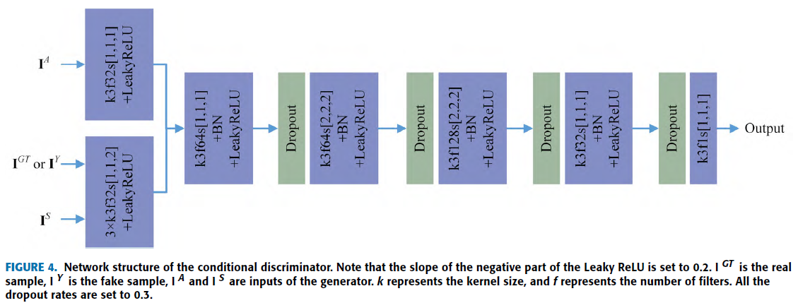
Loss Function
\(G\) 는 generator 라는 의미.
Self-Adaptive Charbonnier Loss
$$L^G_{SC} = \frac{1}{rLWH}\sum_{x,y,z=1,1,1}^{L,W,rH}\sqrt{(I^{GT}{x,y,z}-I^Y {z,y,z})^2+\epsilon}\cdot\bigg(\frac{1}{2}+\frac{(I^{GT}{x,y,z}-I^Y {z,y,z})^2}{2max((I^{GT}-I^Y)^2)}\bigg)$$
3-D Gradient Correction Loss
Charbonnier Loss는 Pixelwise difference에 대한 Loss, Gradient에 대한 손실을 줄 수 있음.
다음과 같이 각 axis에 대한 Gradient 를 이용하여 Loss 제안.
$$L^G_{GC} = \mathbb{E}[(\nabla_{x}I^{GT}{x,y,z} - \nabla {x}I^Y_{x,y,z})^2] \\ + \mathbb{E}[(\nabla_{y}I^{GT}{x,y,z} - \nabla {y}I^Y_{x,y,z})]^2 \\ + \mathbb{E}[(\nabla_{z}I^{GT}{x,y,z} - \nabla {z}I^Y_{x,y,z})^2]$$
$$L^D=\frac{1}{2}\mathbb{E}[(D(I^{GT}, I^A, I^S)-1)^2+D(I^Y, I^A, I^S)^2]$$
$$L^G_{AD}=\mathbb{E}[(D(I^Y, I^A, I^S)-1)^2]$$
\(\ell_2\) Weight Regularization Loss
(Loss는 아니지만…)
Overfitting을 방지하기 위해 사용.
$$L^G_{WR} = \sum\Vert W_G\Vert^2_2$$
3D-Y-Net-GAN Loss
\(L_G = L^G_{SC} + \lambda_1L^G_{GC} + \lambda_2L^G_{AD} + \lambda_3L^G_{WR}\)
3D-DenseU-Net Loss
\(L = L_{SC} + \lambda_1L_{GC} + \lambda_3L_{WR}\)
Experimental Result
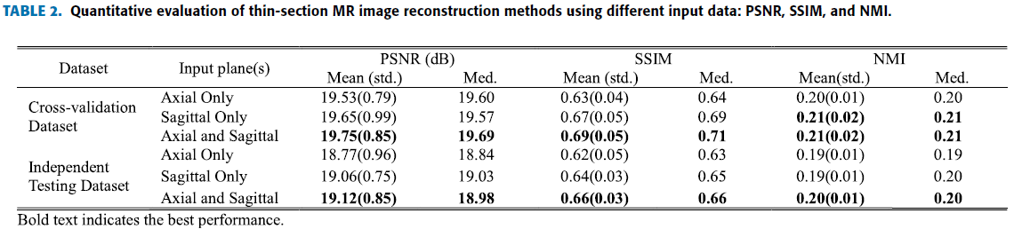
Multiplanar 의 효율성을 검증하기 위해 다음과 같이 세 가지 경우로 나눔.
Axial, Sagittal 둘 다 이용.
Axial 만 이용.
Saigittal 만 이용.
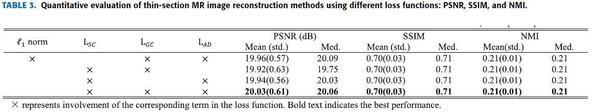
Loss function을 검증하기 위해 네 가지 경우로 나눔.
\(\ell1norm + L_{GC} + L_{AD} + L_{WR}\) (pixelwise loss를 \(\ell1norm\)으로 대체.)
\(L_{SC} + L_{GC} + L_{WR}\)
\(L_{SC} + L_{AD} + L_{WR}\)
\(L_{SC} + L_{GC} + L_{AD} + L_{WR}\)
Evalutaion Method 로는 아래와 같이 네 가지 기법과 자신들의 Network
Metrics으로는 다음 세 가지 사용.
PSNR(Peak Signal-to-Noise Ratio)
$$
\begin{alignedat}{2}
MAX_I = 255 \\
PSNR = 20\cdot\log_{10}\Bigg(\frac{MAX_I}{\sqrt{\frac{1}{rLWH}\sum_{x, y, z}(I^R_{x,y,z}-I^{GT}_{x,y,z})^2}}\Bigg)
\end{alignedat}
$$
SSIM(Structural SIMilarity)
$$L=255(\text{dynamic\ range})$$
$$\mu:\text{Variance} $$
$$\mu_{ab}:\text{Covariance} $$
$$c_1=(k_1L)^2 $$
$$c_2=(k_2L)^2 $$
$$SSIM=\frac{(2\mu_a\mu_b+c_1)(2\sigma_{ab}+c_2)}{(\mu_a^2+\mu_b^2+c_1)(\sigma_a^2+\sigma_b^2+c_2)}$$
NMI(Normalized Mutual Information)
$$H(X) = -\sum_{x_i}\in{X} p(x_i)\log {p(x_i)}$$
$$H(X, Y) = -\sum_{y_i\in{Y}} \sum_{x_i\in{X}}p(x_i, y_i)\log{p(x_i, y_i)}$$
$$NMI(X, Y) = 2\frac{H(X) + H(Y) - H(X, Y)}{H(X)+H(Y)}$$
pixel 값을 [-1, 1]로 clipping -> 다시 8-bit gray scale로 변환.
Generated MR images 와 Ground truth가 비슷할 수록 높은 값을 가짐.
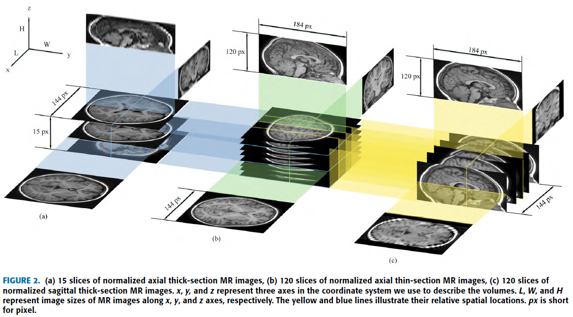
A. Data and Preprocessing
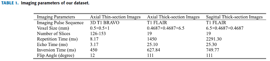
총 154 samples의 2~5세 유아 Axial, Sagittal Thick MRI, Axial Thin MRI
Table 1. 과 같은 parameter 사용.
Dataset 분할
Cross Validation Dataset : 40 samples
Test 1 Dataset : 65 samples
Test 2 Dataset : 49 samples
Preprocessing
각 영상별로 다른 parameter를 가지고 있고 intensities 도 다양하기 때문에 spatial misalignment, intensity imblance를 발견.
Registration을 위해 SPM12 를 이용하여 unified spatial normalization 수행.
DICOM to NIfTI
Segment gray matter, white matter, cerebrospinal fluid, skull, scalp, and air mask.
Nonlinear deformation field
ICBM Asian brain template in affine regularization
Grayscale Normalization
MRI 는 16 bit..
단순 linear transformation 으로 [-1, 1]로 mapping.
Histogram Matching
고정된 샘플을 reference로 histogram matching 적용.
histogram imbalance 제거.
Data Augmentation
Radial Transformation
Mirror Reflection
B. Experimental Settings
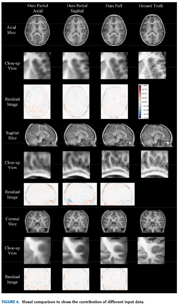
Input을 변경하면서 실험 진행.
Axial 과 Sagittal 을 같이 사용했을 때가 좀 더 세부적인 구조, 적은 왜곡을 보임.
두 축의 영상이 서로 조합하여 reconstruction task를 향상.
Quantitive evaluation 에서도 더 높은 지표를 산출.
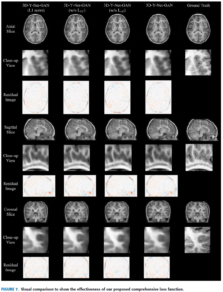
D. Ablation Experiment On Loss Function
Loss를 변경하면서 실험 진행.
Self-Adaptive Charbonnier Loss에 비해 \(\ell1 norm\) 이 흐린 영상을 생성.
Without Gradient Correction Loss
Without Adversarial Loss
덜 realistic 영상을 생성. -> ?????그냥 쓴 말인가..
Table3 …지표 좀 이상..
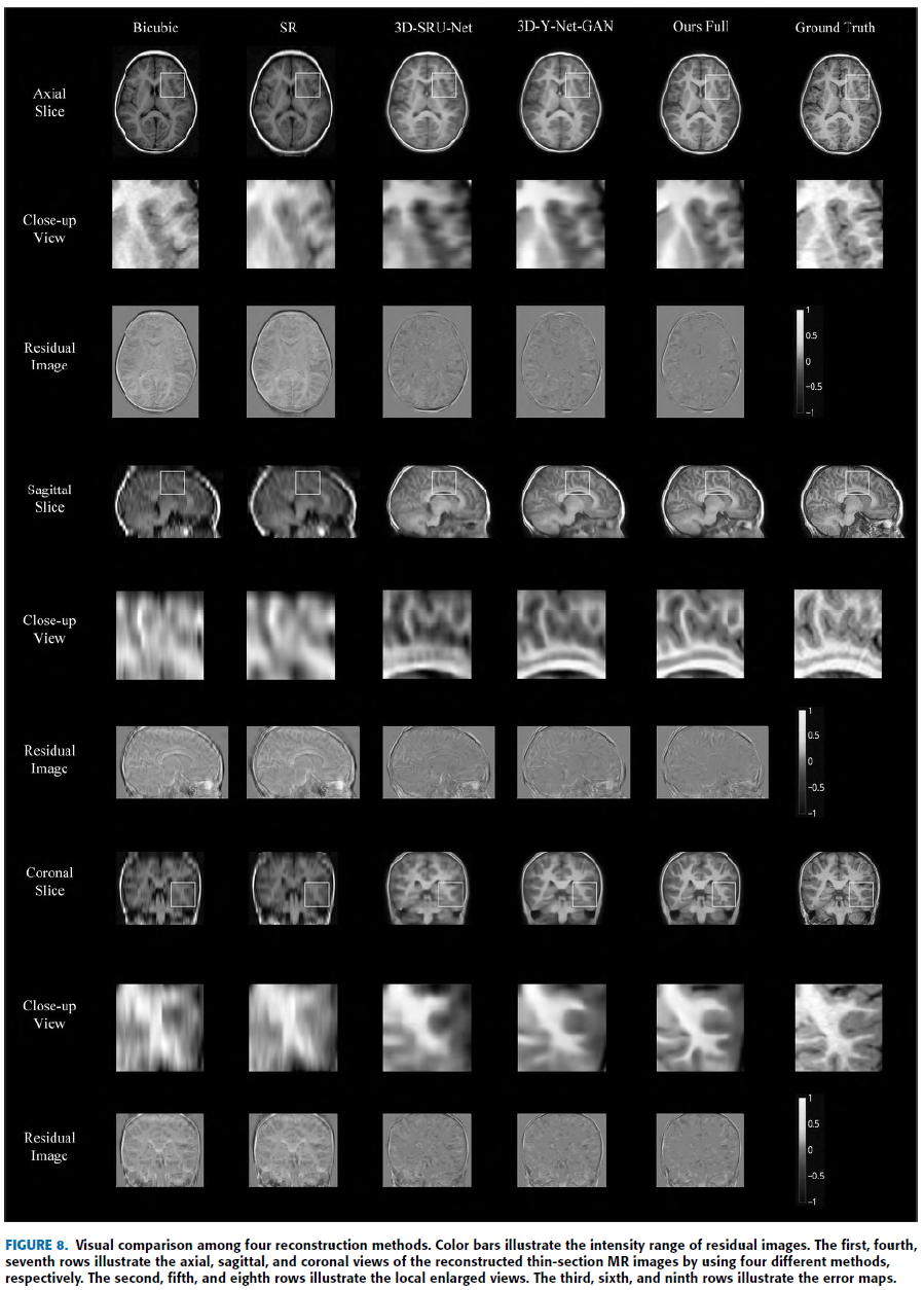
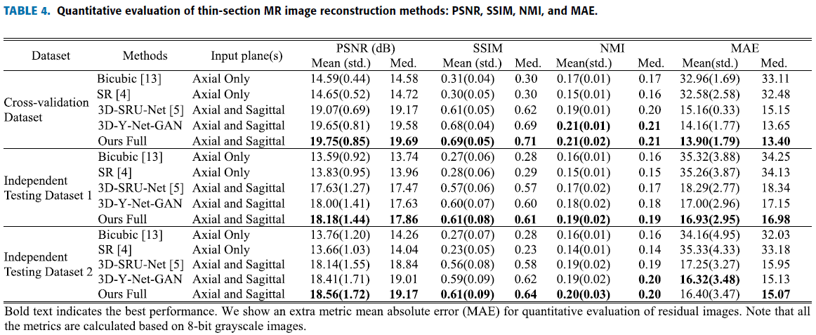
E. Comparison With Other Methods
다른 Method들과 비교.
제안한 method로 생성된 image가 가장 Realistic하고 Ground truth 와 가장 비슷하다고 함.
대부분 Quantitative evaluation 에서 제안한 method가 다른 것들을 다 뛰어넘음.
Conclusion
제안한 Method 에선 Data preprocessing이 매우 중요하다……