preloader
Deep learning

Review: YOLO

You Only Look Once: Unified, Real-Time, Object detection


편의상 bounding box -> bbox

Abstract

  • Object detection을 bboxes, class probabilities regression 문제로 접근.
  • Single Neural Network 로 bboxes와 class probabilities 둘 다 예측.
  • Localization Error가 다소 높지만 background error가 낮음.
  • End-to-End, Extremely fast

1. Introduction

  • Current Detection 시스템
    • DPM : Sliding Window 방식
    • R-CNN 계열 : potential bboxes 추출 -> image 에서 bboxes 부분 다시 classify -> Post-processing
  • Slow, Hard to optimize(각 요소별로 따로따로 학습을 해야함. RPN -> Classifier -> RPN -> …)
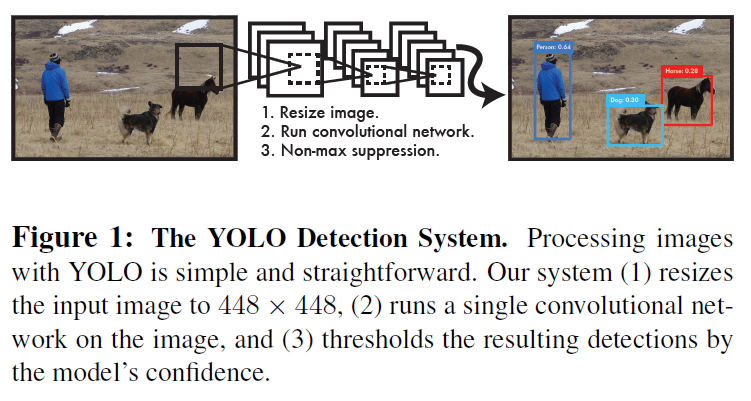
  • 복잡하지 않은 pipeline과 빠른 inferenc time.

    • 45 fps on a Titan X .
  • 이미지 전체를 이용한 prediction

    • Fast R-CNN 보다 적은 background error
  • Object의 general한 representations 학습.

    • natural image로 학습하고 art works로 test 했을 때 기존의 DPM 이나 R-CNN 보다 성능이 좋았다.
    • 새로운 도메인이나 뭔가 모를 입력에 대해 일반화 할 수 있다.

2. Unfied Detection

  • Single Neural Network로 통합.
  • 이미지 전체를 이용해서 각각의 bbox 예측.
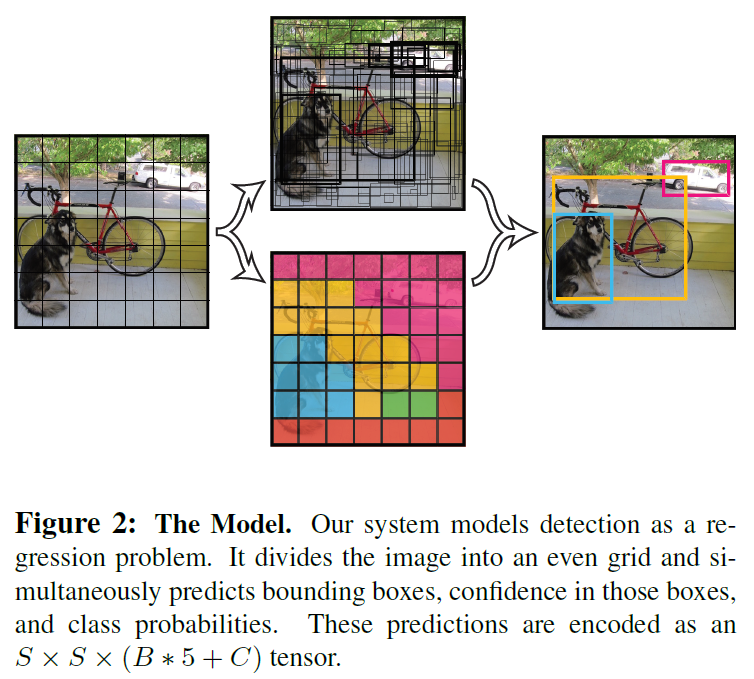
  • 입력 이미지를 S x S grid로 나눔.

    • Feature map이 S x S 라고 이해하면 됨.
  • 각 grid cell은 B개의 bbox의 정보(x, y, w, h, confidence score), 해당 grid cell의 Class probabilities 정보를 가짐.

    • bbox의 정보

      • x, y : bbox의 center 좌표
      • w, h : 이미지 크기에 대비한 상대적인 값.
      • confidence score : bbox가 object를 가졌는지 box가 얼마나 정확히 예측했는지에 대한 score
      • Confidence Score는 다음과 같이 정의. $${Confidence; Score}= Pr(Object) * IOU^{truth}_{pred}$$
      • No object의 경우
        • Confidence Score는 0 이어야함.
      • Confidence Score가 IOU와 같아지길 원함.
    • Class Probabilities 정보

      • C개의 class에 대한 conditional class probabilities, \(Pr(Class_i \mid Object)\)

      • Test 시에는 Conditional class probabilities와 individual box confidence score를 곱했다고 함.
        \(Pr(Class_i|Object) = Pr(Object) * IOU^{truth}_{pred} = Pr(Class_i) * IOU^{truth}_{pred}\)

      • bbox 별로 class confidence score를 알 수 있음.

  • PASCAL VOC 로 평가. S = 7, B = 2, C = 20

  • 최종 출력은 7 x 7 x 30 의 tensor.

2.1 Design

  • 24개의 Convolution layer, 2개의 Fully Connected layer.
  • GoogLeNet의 inception 모듈 대신에 1 x 1 Convolution layer를 이용하여 reduction.
  • Tiny model은 9개의 Convolution layer, 2개의 Fully Connected layer.

2.2 Training

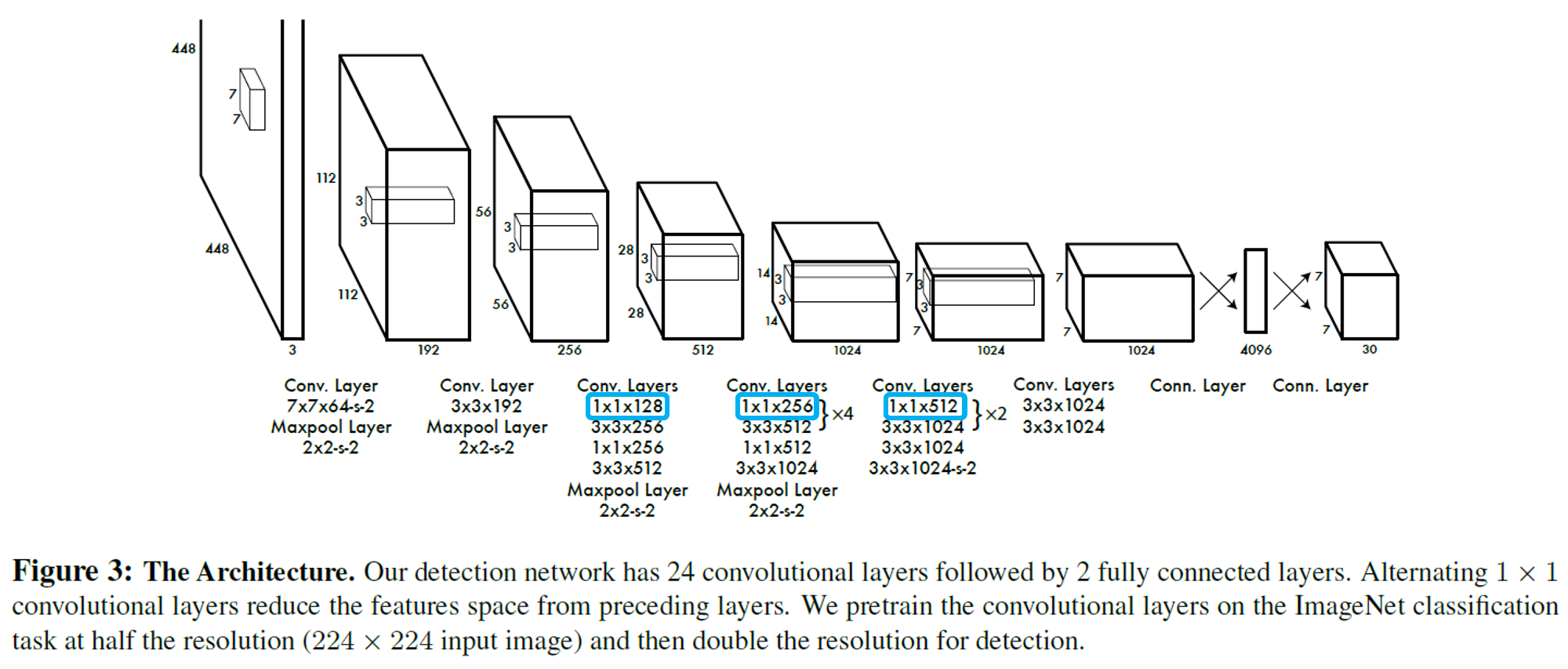
  • 앞 단의 20개의 Convolution layer(Feature Extractor)를 ImageNet 1000-class competition 데이터(224 x 224)로 Pretrain.

  • 20번째 Convolution layer 뒤에 Average Pooling, Fully Connected Layer.

  • ImageNet 2012 validation set으로 top-5 accuracy 88% 정도..

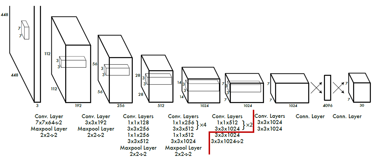
  • Pretrain 후 Detector 부분 추가 후 입력 크기를 448 x 448 로 높여서 학습 진행.

  • Bounding Box의 width, height 값은 이미지의 width, height로 normalize 하여 0 ~ 1 사이 값을 같도록 함.

  • Bounding Box의 x, y 값은 특정 grid cell의 left top으로부터 offset 값. 0 ~ 1 사이 값을 같도록 함.

  • 마지막 layer는 linear activation function 사용.

  • 다른 layer는 leaky ReLU 사용. $$\phi(x)=\begin{cases}x,&if;x >0\\ {0.1}x, & otherwise\end{cases}$$

  • Optimization이 쉬운 Sum-Squared Error 를 사용.

  • 이미지의 대부분 grid cell이 object 를 가지고 있지 않기 때문에 Confidence Score가 0 에 수렴.

  • 이 상황에선 object를 가지고 있는 grid cell의 gradient를 압도할 수 있음.

  • 이를 해결하기 위해 Bbox coordinate loss와 No object의 confidence loss 에 대해 weight 를 부여.
    \(\lambda_{coord} = 5\) and \(\lambda_{noobj} = 0.5\).

  • Sum-Squared Error는 large boxes와 small boxes 를 동일하게 평가.

  • large boxes 에 대해서 중요성을 반영하기 위해 width, height 는 square root 사용.

$$\lambda_{coord}\sum^{S^2}_{i=0}\sum^B_{j=0}\mathbb{I}^{obj}{ij}(x_i-\hat{x}i)^2+(y_i-\hat{y}i)^2$$ $$+\lambda{coord}\sum^{S^2}_{i=0}\sum^B{j=0}\mathbb{I}^{obj}{ij}(\sqrt{w_i}-\sqrt{\hat{w}i})^2 + (\sqrt{h_i}-\sqrt{\hat{h}i})^2$$ $$+ \sum^{S^2}_{i=0}\sum^B{j=0}\mathbb{I}^{obj}{ij}(C_i - \hat{C}i)^2$$ $$ + \lambda{noobj}\sum^{S^2}_{i=0}\sum^B_{j=0}\mathbb{I}^{noobj}_{ij}(C_i - \hat{C}i)^2 $$ $$ + \sum^{S^2}_{i=0}\mathbb{I}^{obj}_{i}\sum^B{c\in{classes}}(p_i(c) - \hat{p}_i(c))^2 $$

  • \(\mathbb{I}^{obj}_{i}\) : Object가 존재하는 Grid Cell i.

  • \(\mathbb{I}^{obj}_{ij}\) : Object가 존재하는 Grid Cell i의 Bounding Box j.

  • Train 관련 Parameter

    • Batch Szie : 64
    • Momentum : 0.9
    • Decay : 0.0005
    • Learning rate
      • \(10^{-3}\) 부터 \(10^{-2}\) 까지 천천히 증가.
      • \(10^{-2}\) 로 75 epochs 학습.
      • \(10^{-3}\) 로 줄여서 30 epochs 학습.
      • \(10^{-4}\) 로 줄여서 30 epochs 학습.
    • Dropout : 0.5
    • Data Augmentation
      • Random Scaling, Translation of up to 20% of the original image size.
      • Random adjustment exposure and saturation

2.3 Inference

  • Large Object 나 여러 grid cell에 걸쳐있는 object는 여러 셀에 predict 될 수 있음.
  • Non-maximal suppression 사용하여 해결.

2.4 Limitations of YOLO

  • 각 Grid Cell은 하나의 클래스만 가질 수 있기 때문에 Grid Cell 하나에 작은 object가 여러 개 있을때 제대로 예측하지 못할 수 있다.
  • 예상치 못한 aspect ratio나 configuration을 가진 객체를 일반화 하는데 어려움.
  • Large box와 Small box를 동일하게 처리.
  • Large box의 small error보다 Small box의 small error가 IOU에 훨씬 큰 영향을 끼침.

3. Comparison to Other Detection Systems

  • 생략

4. Experiments

4.1. Comparison to Other RealTime Systems

  • Fast Yolo는 가장 빠른 속도를 보여줌.
  • YOLO 는 real-time 성능을 보여주면서 mAP도 뛰어난걸 확인할 수 있음.

4.2. VOC 2007 Error Analysis

  • Object Localization은 Fast R-CNN이 더 뛰어남.
  • But, Background Error(False Positive)가 훨씬 높음.

4.3. Combining Fast RCNN and YOLO

  • Fast R-CNN과 YOLO를 앙상블 한 모델이 성능이 가장 좋음.

4.4. VOC 2012 Results

4.5 Generalizability

  • 새로운 도메인, 예상치 못한 입력이 들어왔을때 일반화 성능이 뛰어남.
  • Picasso Dataset 과 People-Art Dataset을 이용하여 다른 모델들과 일반화 성능 비교.
  • YOLO가 가장 성능이 좋은것을 보여줌.
support-btn
도움이 되셨다면 몰랑이에게 밀크티를...!
더 다양한 포스팅을 채우도록 노력할게요!
comments powered by Disqus